
{{ post.title }}
글 편집
글 편집 (이전 에디터)
{{ post.author.name }}
Posted on
| Version | {{ post.target_version }} | Product |
{{ product.name }}
|
|---|---|---|---|
| Tutorial/Manual | {{ post.manual_title }} | Attached File | {{ post.file.upload_filename }} |
- If you can apply the spline data directly to the parameters of the modeling elements, then perform the following procedure.
- If you cannot apply the spline data directly to the parameters of the modeling elements, then you must use an expression to define the spline and apply the data.
This technical tip explains how to use an expression to apply measured spline data to a modeling element (joint or force) in RecurDyn.
Expressions are important modeling elements that enable you to apply mathematical modeling functions as input values. Expressions allow you to use various interpolation functions, such as AKISPL, CUBSPL, and LINSPL, to apply measured spline data to RecurDyn modeling elements. For more details about this procedure, refer to the example in the following video.
Video: Applying Spline Data in RecurDyn
If you are unable to watch this video, click the link below.
Step 1
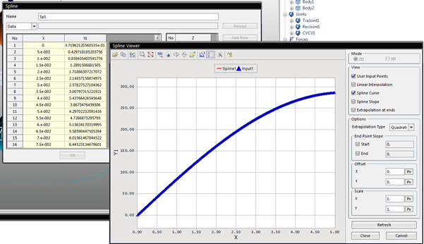
In the RecurDyn menu, on the SubEntity tab, in the Expression group, click Spline. When the Spline dialog window appears, create a spline called Sp1. Sp1 will be used in the expression.
(The following example shows the spline data for a revolute joint motion.)
Step 2
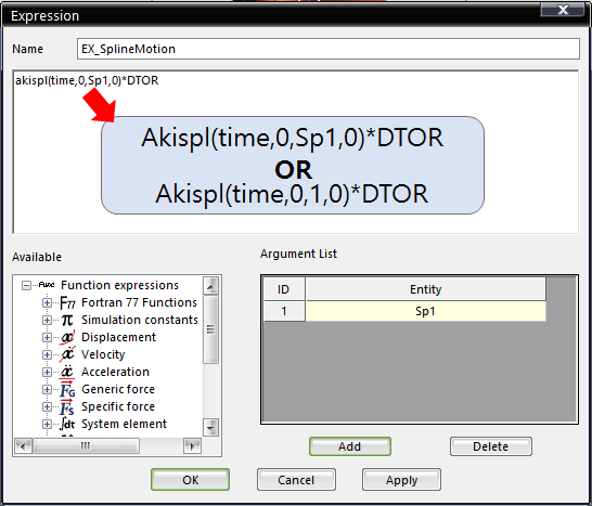
In the Expression dialog window, add the spline (Sp1) to the expression. (This example adds the spline to an AKISPL function.)
- Input: akispl(time, 0, 1, 0) × DTOR
-
Note: DTOR
- This function converts a degree value into a radian value.
- It can be used to apply spline data to modeling elements related to rotation, such as a revolute joint.
Step 3
Apply the expression you created in Step 2 to a joint motion or force to use the spline data in the element during analysis.

<Caution>
If the x value exceeds the limit defined in the spline, it will be replaced with an extrapolated value.
(For example, if the x value is time, then the End Time in the simulation settings cannot exceed the range of the x value.)
<Note> AKISPL Function

Argument Definitions
- X: An input variable for the AKISPL function. Generally, this variable is time or a function that returns a real number. It corresponds to the x value of the spline function.
- Z: An input variable for the AKISPL function. In three dimensional spline functions, this is the second independent variable. This variable must be a function that returns a real number. Otherwise, 0 is applied. In other words, the spline consists of only the x and y axes.
- Curve name: The name or argument number of the spline data defined on the SubEntity tab. Enter the name of the spline that you want to use (Sp1 in the above example) or register the spline in the Argument List and enter its numerical ID.
-
Order: Defines how to interpolate the function.
- 0: Returns the function as it is.
- 1: Returns the first derivative of the function.
- 2: Returns the second derivative of the function.
Formulation
