FunctionBay Technical Support Site | Solver – Becoming an Experienced User #5

Version	{{ post.target_version }}	Product	{{ product.name }}
Tutorial/Manual	{{ post.manual_title }}	Attached File	{{ post.file.upload_filename }}

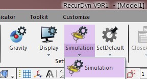
RecurDyn provides various options (Simulation Parameters).

[Home]-[Setting]-[Simulation]

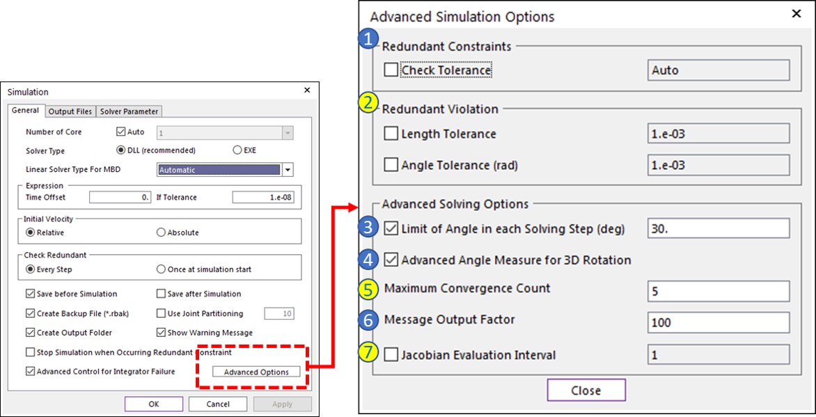
In most of the cases, you can use the default values as they are. But sometimes you may need to change the options.

In this article, brief explanation about each options will be described. You can refer to the manual for the details.

Yellow ones are the parameters used frequently.

For the basic solver parameters, please refer to the below articles.

1. Check Tolerance

In general, the default (OFF) would be good enough.
This option is used as a numerical tolerance when the solver judge the redundant constraint internally.
If this value is changed, Solver can judge the different constraint as a redundant constraint. (the DOF which was regarded as a redundant constraint can be treated as not a redundant constaint.)

2. Redundant violation

It is recommended to use this option as ON. But you can use the default value, 0.001 as it is.
RecurDyn automatically judges the Redundant constraint so that the over-constrained model can be simulated easily. But sometimes it can cause the unintended result because of the over-constraint. (usually it is a user error)
For example, a revolute joint is regarded as a redundant constraint, so the action marker and the base marker can be apart. But if the user defined a revolute joint, it means the user may not want those markers not to be separated.
If this option, Redundant violation is used, when the DOF regarded as a redundant constraint is apart or rotated more than the defined value, the solver treats it as an error and stops.
It is easier to understand to watch the below video.

In this video, 2 motions were defined to the 4-bar linkage intentionally. So the revolute joint (up-left) is regarded as a redundant constraint, and 2 bodies are apart. But the user may not want this result.
If redundant violation option is used as ON, the solver stops when the constraint regarded as a redundant constraint is apart or rotated becuase it is treated as an error.
This can help the user to find the unintended mistake.
If this is a model which needs long time for simulation, user can save the time which can be wasted!

3. Limit of Angle in each Solving Step (deg)

In general, the default (ON) would be good enough.
But if you load the model saved by RecurDyn V8R5 or the previous version, this option is OFF, so it is recommended to check it ON.
This is very useful for the model which involves high speed rotation.
Too fast rotation can cause the inaccurate result. This option limits the angle of the rotation during one step so that it reduces the step size to improve the accuracy.
So, even if the user use the big max. step size, the solver adjust the step size according to the amount of the rotation, so that it gives the positive effect on the simulation speed.

4. Advanced Angle Measure for 3D Rotation

In general, the default (ON) would be good enough.
But if you load the model saved by RecurDyn V8R5 or the previous version, this option is OFF, so it is recommended to check it ON.
From RecurDyn V9R1, the algorithm to calculate the rotation of a Bushing force or a matrix force has been improved, which is used when this option is ON.
In case of a Bushing force, if you don't use this option (OFF), for the X, Y axes, only the rotation smaller than 90 degrees was allowed, but there is no such limitation if you use this option (ON) (Related Post )
Especially, this option improved the usage of the bushing force, which is frequently used to remove the redundant constraint or to get the reaction force distributed across the several joints.

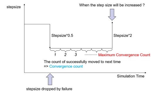
5. Maximum Convergence Count

RecurDyn solver increase the step size to make the simulation speed faster when the convergence is stable.
This option means the count of the successful convergence to decide if the step size can be increased.
If this value is 1, then just 1 successful convergence increases the step size, so that the simulation speed can become faster. But it can cause instability of the simulation as a side effect.
For example, if you need many repetitive simulation such as DOE, firstly make a stable and accurate enough model. then try the smaller number for this option and compare the simulation results. If you can get the good enough result in less simulation time, it means you can use the smaller Maximum Convergence Count.

6. Message Output Factor

During simulation, the solver information such as TIME, STEPSIZE, A_DELNRM, ... are written in the message window.
This option is about how frequently the information is written, so you can use the default value in general.
But when the step size is too small, it can be inconvenient because of too much information. You can reduce the frequency of displaying those information by increasing the factor ( > 1000)
This option doesn't affect the simulation result at all.

7. Jacobian Evaluation Interval

This option controls the frequency to calculate the Jacobian during simulation.
If the change of the behavior of the model is not big, the simulation speed can be improved by using the bigger interval. (> 1)
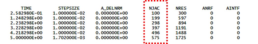
NJAC written in the message window means the accumulated number of the Jacobian evaluation.
In the below case, 100->199 means the Jacobian was calculated 99 times. If this variation is similar to the Message Output Factor (the default is 100), we can assume that Jacobian doesn't change a lot. In this case, the simulation speed can be improved by using the bigger Jacobian Evaluation Interval. (But it can lower the accuracy, so you need to be careful when you change this value)
For example, if you need many repetitive simulation such as DOE, firstly make a stable and accurate enough model. then try the bigger number for this option and compare the simulation results. If you can get the good enough result in less simulation time, it means you can use the bigger Jacobian Evaluation Interval.